Analyzing DNS Data with SVD and DMD
In this project, I explored the use of Singular Value Decomposition (SVD) and Dynamic Mode Decomposition (DMD) to analyze fluid dynamics data obtained from Direct Numerical Simulations (DNS). DNS provides highly detailed and complex data for simulating turbulent flows, making it an ideal dataset to apply these decomposition techniques.
Motivation
DNS data is rich but also computationally intensive to handle due to its high dimensionality. Reducing this complexity while retaining the essential features of the flow is key for developing efficient models. This is where techniques like SVD and DMD come into play.
- SVD helps in breaking down the data into orthogonal components, which allows us to identify the dominant structures or modes in the flow field.
- DMD provides insights into the temporal evolution of these structures, enabling us to study the dynamics and predict future states of the system.
Approach
The DNS dataset consisted of high-resolution velocity fields sampled over time. Before applying SVD and DMD, the data had to be processed to ensure consistency and eliminate noise. I began by normalizing the data and reshaping the snapshots into a 2D matrix where each column represented a snapshot in time, and each row corresponded to a spatial point.
SVD was applied to decompose the DNS dataset into its spatial modes, singular values, and temporal coefficients. This allowed me to rank the modes by their energy contribution to the overall flow. The singular values were used to determine the importance of each mode, with the highest-ranking modes capturing the most significant flow structures.
U, Sigma, Vt = np.linalg.svd(data_matrix, full_matrices=False)- U (left singular vectors): Represent the spatial modes.
- \(\Sigma\) (singular values): Indicate the energy associated with each mode.
- Vt (right singular vectors): Capture the temporal dynamics of each mode.
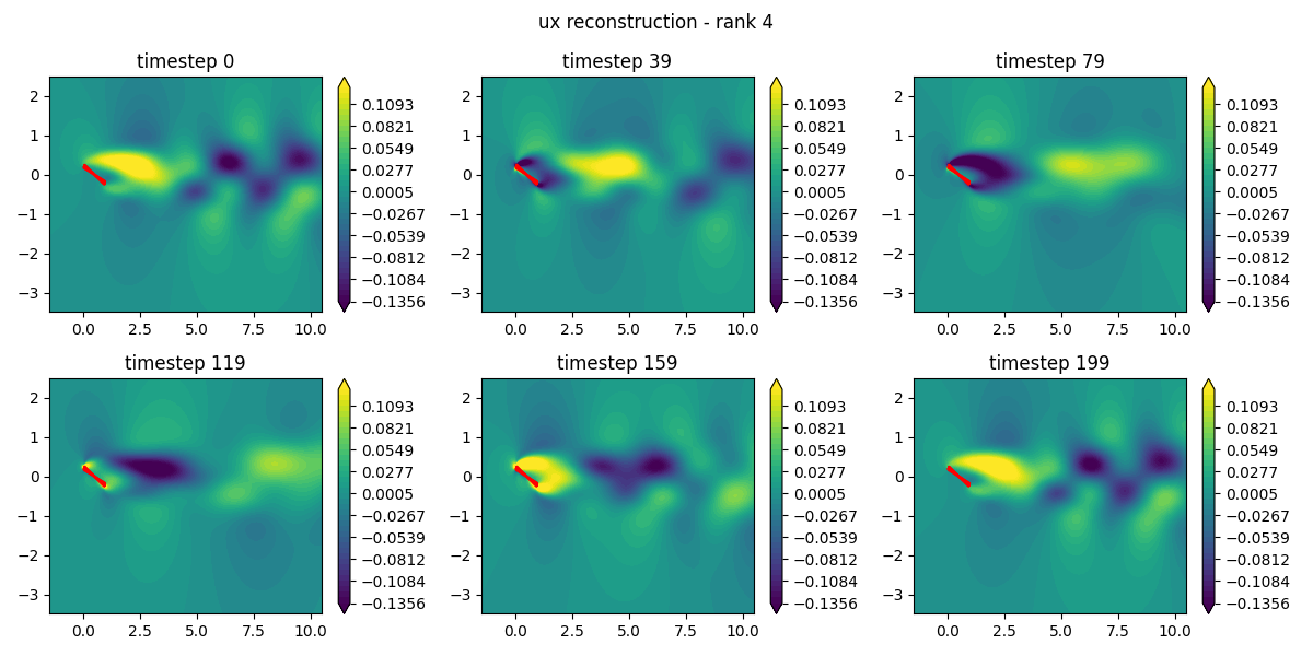
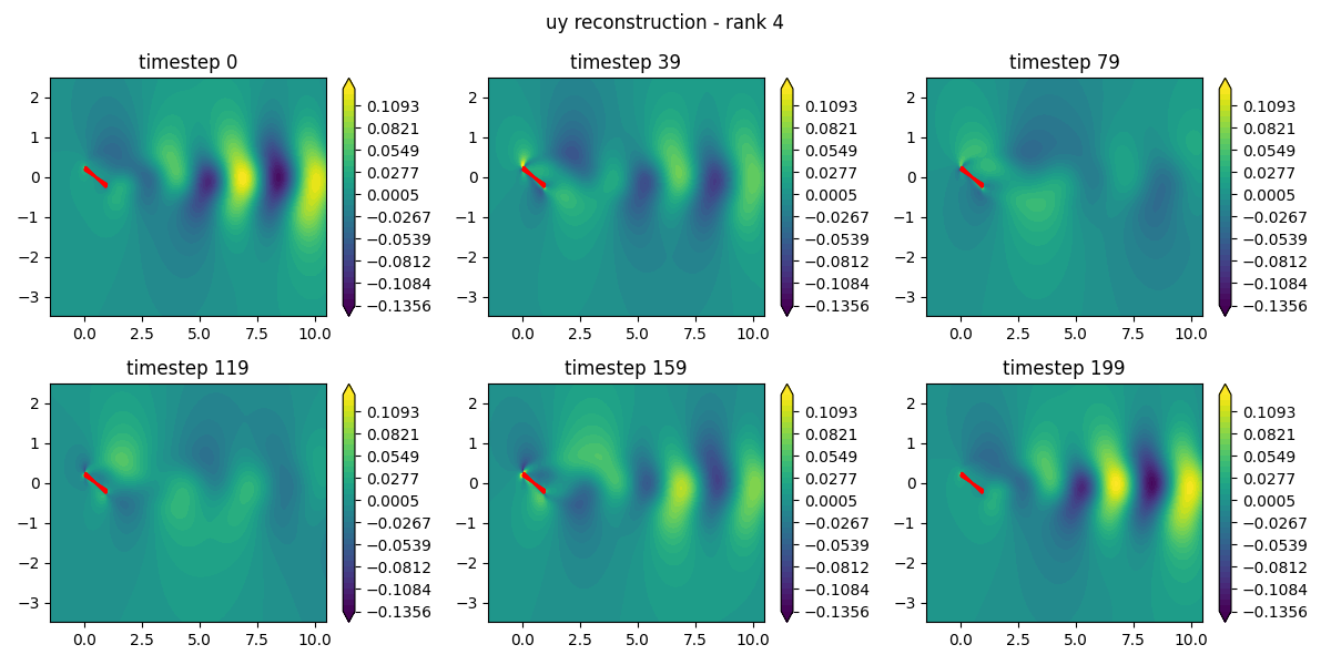
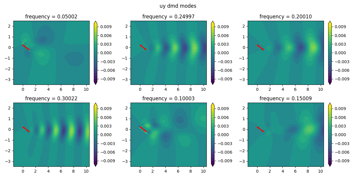
DMD was then applied to analyze the time evolution of the flow. Unlike SVD, which is purely a spatial decomposition, DMD links the spatial structures to their temporal dynamics, identifying coherent structures that evolve over time.
# DMD implementation (using an external library like PyDMD)
dmd = DMD(svd_rank=5)
dmd.fit(X=data_matrix)
modes = dmd.modes
frequencies = dmd.frequencies
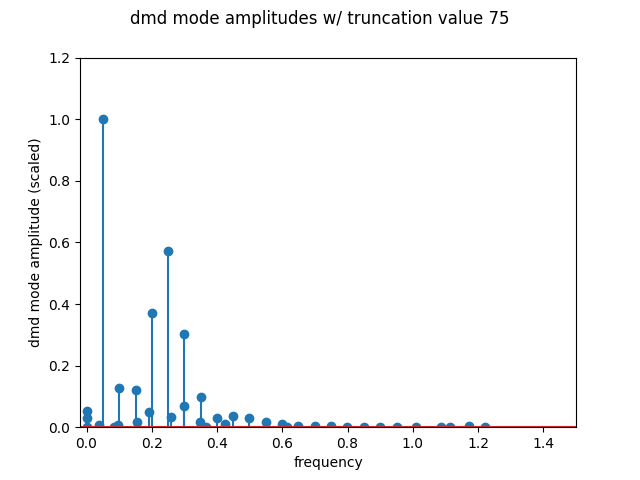
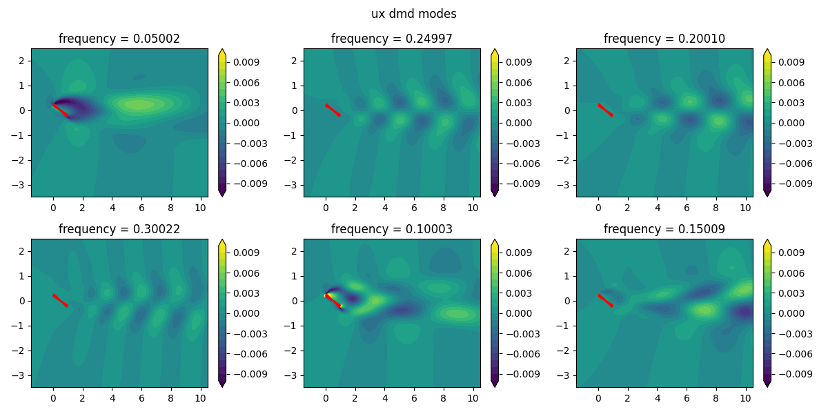
Through DMD, I was able to extract dynamic modes corresponding to specific temporal frequencies, providing insights into oscillatory behavior within the flow field. These modes offered a deeper understanding of the flow’s transient behavior.
Results
The SVD analysis revealed that the first few modes captured over 90% of the system’s energy, enabling us to approximate the flow with a low-dimensional representation. The DMD analysis provided detailed insights into how these modes evolve over time, helping to predict future flow states based on the dynamics.
Key findings include:
- The dominant mode captured the largest coherent structure in the flow, representing the main flow features.
- Higher-order modes revealed finer, less energetic structures that contributed to turbulent fluctuations.
- DMD frequencies corresponded to specific flow instabilities and oscillatory patterns, giving us predictive power over the system’s temporal behavior.