Diffusion-Based Trajectory Generation in Maze Environments
Trajectory planning in cluttered environments is traditionally framed as a search or optimization problem. Given a map, a start, and a goal, classical planners explicitly reason about feasibility by expanding a graph or sampling the configuration space. In this project, I explored a different perspective: treating trajectory planning as a conditional generative modeling problem, and using diffusion models to represent distributions over entire trajectories rather than producing actions step by step.
I considered navigation in a fixed two-dimensional maze, conditioned only on start and goal locations, with no explicit map information provided to the model at inference time. The objective was not to beat classical planners, rather, I wanted to understand what diffusion models learn when applied to a structured planning problem with hard geometric constraints.
Problem Setup
The environment is a single binary occupancy grid representing a maze generated via recursive depth-first search backtracking. Start and goal locations are sampled uniformly from free cells. Demonstration trajectories are generated by running breadth-first search on the grid to compute shortest paths, which are then resampled to a fixed horizon and normalized to lie in \([-1, 1]\).
Each trajectory is represented as a sequence of two-dimensional coordinates, and the diffusion model is trained to generate trajectories conditioned only on the start and goal states. Because the environment is fixed across the dataset, obstacle avoidance must be learned implicitly from demonstrations and from an auxiliary training signal rather than from explicit map conditioning.
Network Architecture and Evaluation
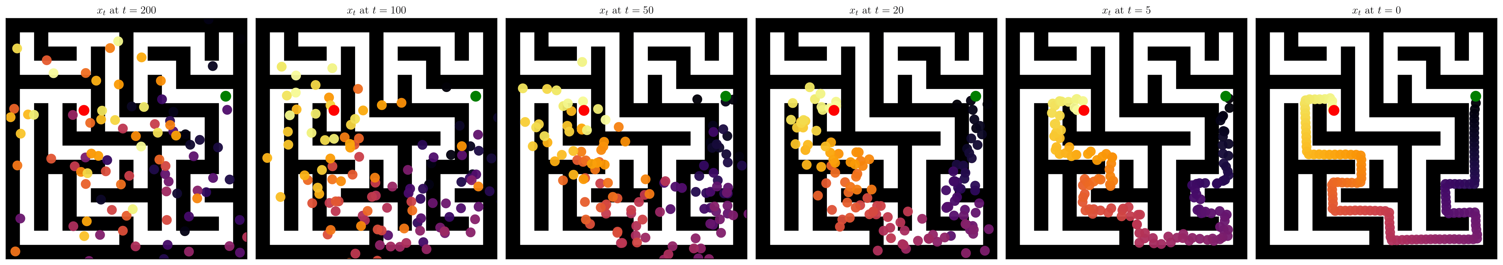
Trajectory generation is modeled using a denoising diffusion probabilistic model operating directly on fixed-length trajectories. A forward diffusion process progressively corrupts demonstration trajectories with Gaussian noise, while a learned reverse process denoises them step by step. Sampling from the model corresponds to synthesizing an entire trajectory in a single generative rollout.
The denoising network is implemented as a temporal U-Net, treating time as the primary convolutional axis and spatial coordinates as channels. Conditioning on the start and goal is provided through a learned embedding that is injected at every layer. This architecture allows the model to capture both local smoothness and long-range temporal structure along the trajectory.
One of the appealing aspects of this formulation is that it naturally produces smooth, temporally coherent trajectories without requiring an explicit planner at inference time. However, the diffusion objective alone does not enforce feasibility with respect to obstacles.
To bias the model toward feasible behavior, I augmented the diffusion loss with a differentiable collision penalty applied during training. The maze occupancy grid is treated as a scalar field, and continuous trajectory points are evaluated against it using bilinear interpolation. To reduce missed collisions between sparse waypoints, trajectories are densified prior to collision evaluation.
The collision loss is computed on the model’s estimate of the clean trajectory at each diffusion step, rather than on the noisy input. This provides gradient information that encourages the denoiser to move trajectories toward free space over the course of training. Importantly, this penalty acts as a soft regularizer rather than a hard constraint, and collision avoidance at inference time remains approximate and probabilistic.
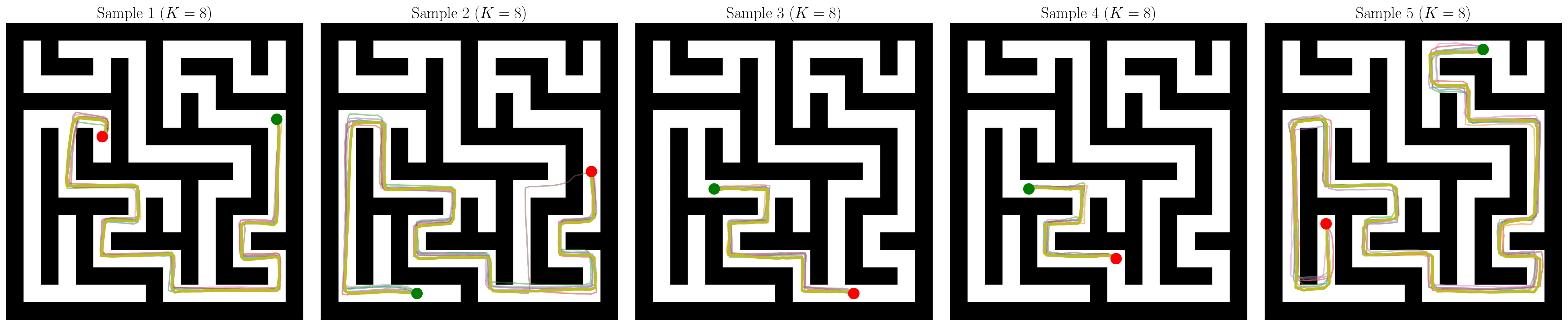
At evaluation time, the model generates multiple candidate trajectories for a given start–goal pair by sampling from the reverse diffusion process. Because individual samples may still intersect obstacles, I adopted a simple best-of-\(K\) selection strategy. Each candidate is scored using the same differentiable collision metric used during training, and the trajectory with the lowest collision score is selected.
Qualitative results show that this procedure substantially improves feasibility. Even when some samples collide with walls, it is often the case that at least one trajectory in the set avoids obstacles almost entirely. The following figure shows several examples, illustrating both the variability of individual samples and the effect of best-of-\(K\) selection.
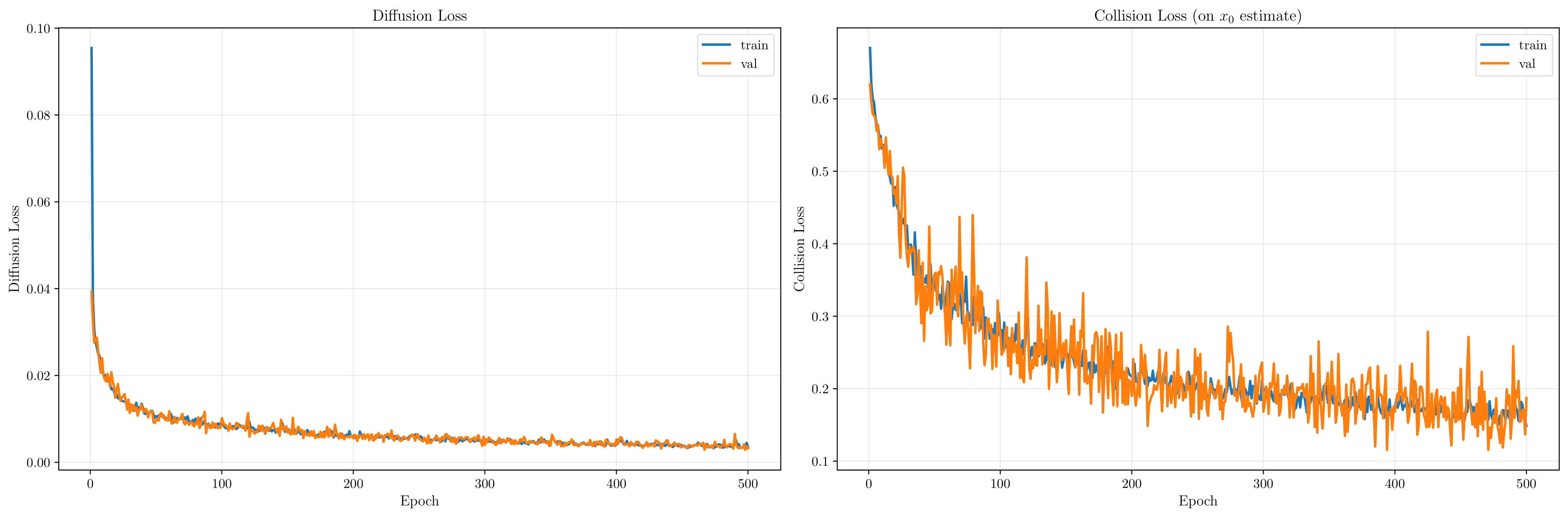
The diffusion loss converges rapidly, indicating that the model quickly learns to match the distribution of demonstration trajectories. In contrast, the collision loss decreases more slowly and remains nonzero, reflecting the soft nature of the collision surrogate.
This behavior is visible in the generated trajectories, which often hug corridor walls or graze obstacles. Numerically, these trajectories incur low collision penalties, even if they appear visually close to walls. This highlights a fundamental limitation of using smooth, differentiable surrogates to approximate hard geometric constraints.